Getting started with Pycea

Pycea provides a suite of tools for analyzing and visualizing phylogenetic trees. This tutorial will walk you through the basics of using Pycea.

import pycea as py
import scanpy as sc
import matplotlib.pyplot as plt

plt.rcParams["figure.figsize"] = (4, 4)

TreeData object

Pycea is designed to work with the treedata.TreeData, a wrapper around anndata.AnnData that adds two additional attributes, obst and vart, for storing trees of observations and variables. To learn more about TreeData, take a look at the getting started guide.

For this tutorial, we will use a TreeData containing a single tumor from the KP mouse lineage tracing dataset published by Yang, Jones, et al. 2022.

tdata = py.datasets.yang22()
tdata

TreeData object with n_obs × n_vars = 1109 × 2000
    obs: 'tumor', 'mouse', 'lane', 'fitness', 'plasticity', 'cluster', 'tree'
    var: 'highly_variable', 'means', 'dispersions', 'dispersions_norm'
    uns: 'priors'
    obsm: 'X_scVI', 'X_umap', 'characters'
    layers: 'counts'
    obst: '3435_NT_T1'

Here obst contains a single lineage tree named 3435_NT_T1, which is represented as a networkx.DiGraph.

print(tdata.obst["3435_NT_T1"])

DiGraph with 1890 nodes and 1889 edges

Plotting basics

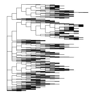
Pycea implements an intuitive plotting language where complex plots can be built from simple components. The first step is to render the branches using pycea.pl.branches().

py.pl.branches(tdata);

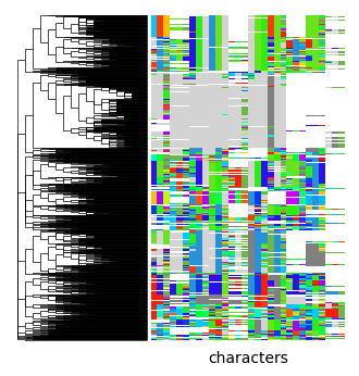
pycea.pl.annotation() adds leaf annotations to a plot, such as the indels used to reconstruct the lineage tree, which are stored in tdata.obsm["characters"]. Here we use pycea.get.palette() to generate an indel color palette and specify that branches should be extended.

indel_palette = py.get.palette(
    tdata,
    "characters",
    custom={"-": "white", "*": "lightgrey"},
    cmap="gist_rainbow",
    priors=tdata.uns["priors"],
    sort="random",
    random_state=0,
)
py.pl.branches(tdata, extend_branches=True)
py.pl.annotation(tdata, keys="characters", palette=indel_palette);

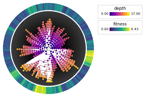
pycea.pl.nodes() renders node data on a plot. For example, we can render a polar tree with internal nodes colored by their depth and leaves annotated with their estimated phylogenetic fitness from Yang, Jones, et al. 2022.

py.pl.branches(tdata, extend_branches=True, polar=True)
py.pl.nodes(tdata, color="depth", cmap="plasma")
py.pl.annotation(tdata, keys="fitness", cmap="viridis", width=0.2)

<PolarAxes: >

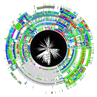
For convenience, Pycea also implements pycea.pl.tree() which combines the above functions. pycea.pl.tree() is useful for quickly visualizing a tree, but does not provide the same flexibility as plotting components individually.

py.pl.tree(tdata, keys="characters", extend_branches=True, polar=True);

Scanpy integration

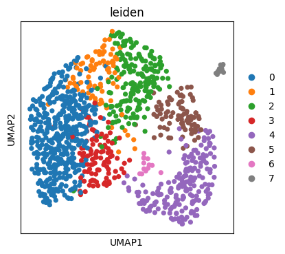
Since treedata.TreeData is a wrapper around anndata.AnnData, it is fully compatible with the Scverse ecosystem and can be used wherever anndata.AnnData is used. For example, we can use Scanpy to generate a UMAP embedding of the malignant cells’ transcriptional state, colored by leiden cluster.

sc.tl.pca(tdata)
sc.pp.neighbors(tdata)
sc.tl.leiden(tdata, resolution=0.7, flavor="igraph")
sc.tl.umap(tdata, random_state=0)
sc.pl.umap(tdata, color="leiden")

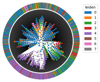
We can directly analyze and plot the leiden clusters with Pycea. Here we will infer the leiden cluster of internal nodes using pycea.tl.ancestral_states() and then plot these on the tree.

py.tl.ancestral_states(tdata, keys="leiden", method="fitch_hartigan")
py.pl.branches(tdata, polar=True, extend_branches=True)
py.pl.nodes(tdata, color="leiden", legend=False)
py.pl.annotation(tdata, keys="leiden", width=0.2, cmap="tab20");

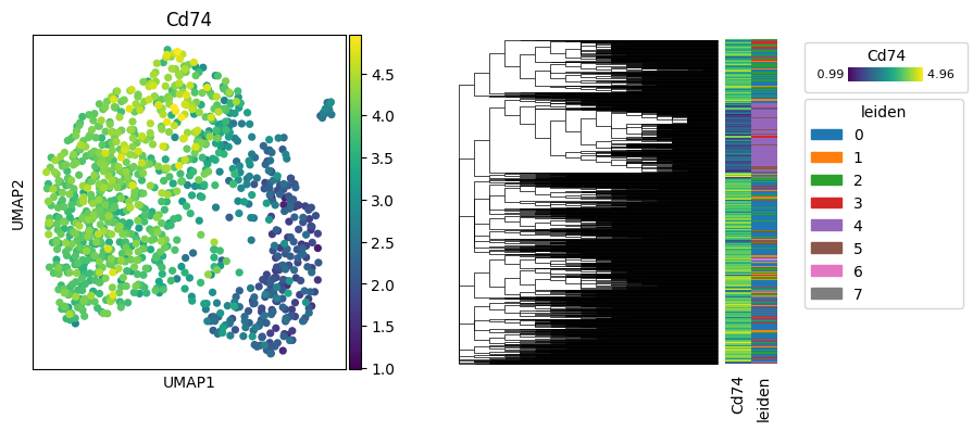
Expression heritability

Malignant cell expression clearly varies by position in the tree but what specific genes drive these differences? One way to investigate this is by calculating the heritability of each gene’s expression across the tree using the pycea.tl.autocorr() function. We first identify the 10 closest relatives for each cell then calculate the Moran’s I statistic for each gene with respect to the graph structure.

py.tl.tree_neighbors(tdata, n_neighbors=10)
heritability = py.tl.autocorr(tdata, method="moran", copy=True)
heritability.sort_values("autocorr", ascending=False).head(10)

	autocorr	pval_norm	var_norm
Cd74	0.591382	0.0	0.000058
Ly6k	0.500966	0.0	0.000058
Krt20	0.496902	0.0	0.000058
H2-Ab1	0.451960	0.0	0.000058
Gsto1	0.451174	0.0	0.000058
Cd24a	0.442243	0.0	0.000058
Plac8	0.426849	0.0	0.000058
Onecut2	0.424653	0.0	0.000058
S100a6	0.412787	0.0	0.000058
H2-Aa	0.412742	0.0	0.000058

Cd74 has the highest Moran’s I value, indicating significant heritability. We’ll visualize its expression on the tree and the UMAP embedding.

fig, axes = plt.subplots(1, 2, figsize=(9, 4))
sc.pl.umap(tdata, color=["Cd74"], ax=axes[0], show=False)
py.pl.tree(tdata, keys=["Cd74", "leiden"], extend_branches=True, annotation_width=0.1, ax=axes[1])

<Axes: >

Clades and subsetting

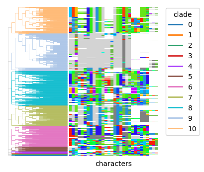
pycea.tl.clades() can be used to identify clades within the tree. For example, it can label clades formed by cutting the tree at a specified depth, such as depth=1.

py.tl.clades(tdata, depth=1)
py.pl.branches(tdata, extend_branches=True, color="clade")
py.pl.annotation(tdata, keys="characters", palette=indel_palette);

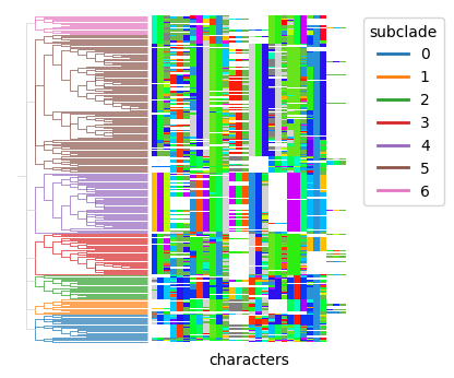
We can then subset the treedata.TreeData object to focus on a specific clade and identify subclades within it.

subset_tdata = tdata[tdata.obs["clade"] == "8"].copy()
py.tl.clades(subset_tdata, depth=2, key_added="subclade")
py.pl.branches(subset_tdata, extend_branches=True, color="subclade")
py.pl.annotation(subset_tdata, keys="characters", palette=indel_palette);

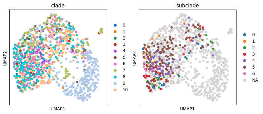
Conveniently, these clades are stored in tdata.obs so we can plot them on the UMAP embedding.

tdata.obs["subclade"] = subset_tdata.obs["subclade"]
sc.pl.umap(tdata, color=["clade", "subclade"])

Learning more

This tutorial just scratches the surface of what you can do with Pycea. To learn more about Pycea’s capabilities check out the full API.

If you have any questions or feedback, please reach out by submitting an issue on GitHub.